PCA via SVD and via AffinityMatcher

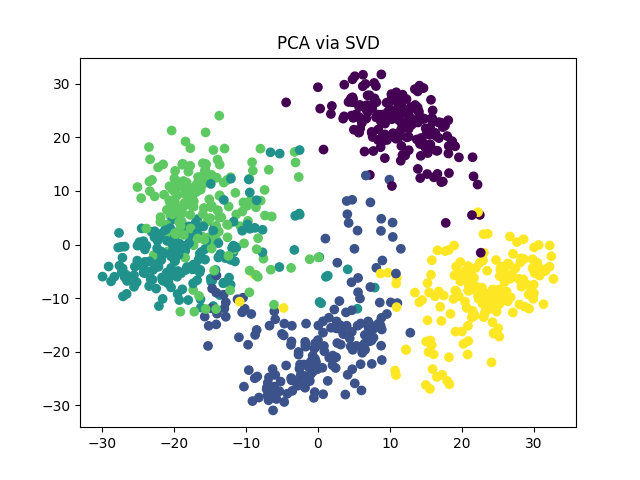
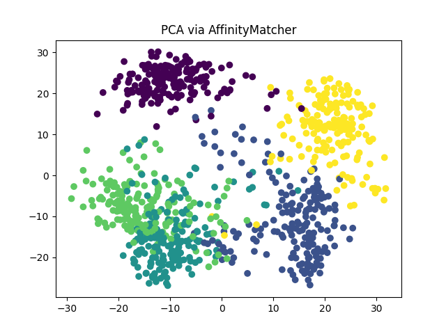
We show how to compute a PCA embedding using the closed form and using the AffinityMatcher class. Both approaches lead to the same solution.

# Author: Hugues Van Assel <vanasselhugues@gmail.com>
#
# License: BSD 3-Clause License

import matplotlib.pyplot as plt
from sklearn.datasets import load_digits

from torchdr import AffinityMatcher, ScalarProductAffinity
from torchdr.spectral import PCA

Load toy images

First, let’s load 5 classes of the digits dataset from sklearn.

digits = load_digits(n_class=5)
X = digits.data
X = X - X.mean(0)

PCA via SVD

Let us perform PCA using the closed form solution given by the Singular Value Decomposition (SVD). In Torchdr, it is available at torchdr.PCA.

Z_svd = PCA(n_components=2).fit_transform(X)

plt.figure()
plt.scatter(Z_svd[:, 0], Z_svd[:, 1], c=digits.target)
plt.title("PCA via SVD")
plt.show()

PCA via AffinityMatcher

Now, let us perform PCA using the AffinityMatcher class torchdr.AffinityMatcher as well as the scalar product affinity torchdr.ScalarProductAffinity for both input data and embeddings, and the square loss as global objective.

model = AffinityMatcher(
    n_components=2,
    affinity_in=ScalarProductAffinity(),
    affinity_out=ScalarProductAffinity(),
    loss_fn="square_loss",
    init="normal",
    lr=1e1,
    max_iter=50,
    backend=None,
)
Z_am = model.fit_transform(X)

plt.figure()
plt.scatter(Z_am[:, 0], Z_am[:, 1], c=digits.target)
plt.title("PCA via AffinityMatcher")
plt.show()

We can see that we obtain the same PCA embedding (up to a rotation) using both methods.