Entropic Affinities can adapt to varying noise levels

We show the adaptivity property of entropic affinities on a toy simulated dataset with heteroscedastic noise.

# Author: Hugues Van Assel <vanasselhugues@gmail.com>
#
# License: BSD 3-Clause License

import torch
import matplotlib.pyplot as plt
from matplotlib import cm

from torchdr import (
    NormalizedGaussianAffinity,
    EntropicAffinity,
)

We generate three Gaussian clusters of points with different standard deviations (respectively std=1, 2 and 3).

torch.manual_seed(0)
n_cluster = 20  # number of points per cluster

X1 = torch.Tensor([-10, -10])[None, :] + torch.normal(
    0, 1, size=(n_cluster, 2), dtype=torch.double
)
X2 = torch.Tensor([10, -10])[None, :] + torch.normal(
    0, 2, size=(n_cluster, 2), dtype=torch.double
)
X3 = torch.Tensor([0, 10])[None, :] + torch.normal(
    0, 3, size=(n_cluster, 2), dtype=torch.double
)

X = torch.cat([X1, X2, X3], 0)


def plot_affinity_graph(G):
    m = G.max().item()
    for i in range(3 * n_cluster):
        for j in range(i):
            plt.plot(
                [X[i, 0], X[j, 0]],
                [X[i, 1], X[j, 1]],
                color="black",
                alpha=G[i, j].item() / m,
            )

Row-normalised Gaussian affinity with constant bandwidth

We first consider a Gaussian affinity, normalized by row, with a constant bandwidth. Such a global bandwidth only controls the global entropy of the affinity.

In TorchDR, we can easily implement it using torchdr.NormalizedGaussianAffinity and setting the parameter normalization_dim=1.

aff = NormalizedGaussianAffinity(
    sigma=1, normalization_dim=1, keops=False, zero_diag=False
)
K = aff(X)

plt.figure(1, (6, 3))

plt.subplot(1, 2, 1)
plt.imshow(K, cmap=cm.Blues)
plt.title("Gaussian Affinity Matrix")

plt.subplot(1, 2, 2)
plot_affinity_graph(K)
plt.scatter(X[:, 0], X[:, 1], alpha=0.5)
plt.title("Gaussian Affinity Graph")
plt.show()

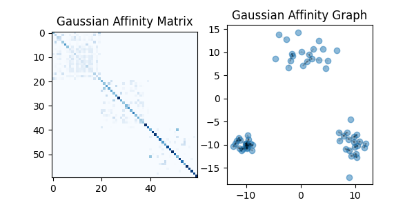
We can observe a remarkable heterogeneity in the density of connections. This occurs because it is less costly to create connections in high-density regions. As a consequence, points in sparse regions create very few connections with their neighbors.

Entropic affinity (adaptive bandwidth)

To remedy this issue, we can use an entropic affinity. The entropic affinity employs an adaptive bandwidth that depends on the local density of points. By controling the entropy of each row of the affinity matrix, it ensures that each point has the same number of effective neighbors (given by the perplexity parameter) regardless of the local density around it.

In TorchDR, this object is available here : torchdr.EntropicAffinity.

aff_ea = EntropicAffinity(
    perplexity=5, keops=False, verbose=False, zero_diag=False, sparsity=False
)
EA = aff_ea(X)

plt.figure(1, (6, 3))

plt.subplot(1, 2, 1)
plt.imshow(EA, cmap=cm.Blues)
plt.title("Entropic Affinity Matrix")

plt.subplot(1, 2, 2)
plot_affinity_graph(EA)
plt.scatter(X[:, 0], X[:, 1], alpha=0.5)
plt.title("Entropic Affinity Graph")
plt.show()

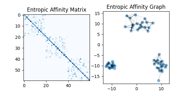
We can now observe a homogeneous density of connections across clusters. Thus, the entropic affinity effectively filters out the various noise levels.

This affinity is an important component of the TSNE algorithm.